My research is primarily focused on Optimal Control, Nonlinear and Hybrid Systems, Analytical Mechanics and Chaos, with applications in Automotive, Sensors and Actuators and Robotics. In the following, an introductory text is provided for each of my areas of research.
1) Classical Optimal Control Theory:
Show Description/Hide
Optimal control deals with the problem of finding a control law for a given system such that a certain optimality criterion is achieved. An optimal control problem includes a cost functional in the form of
$$
J = \int_{t_{0}}^{t_{f}} l\left(x,u,t\right)dt + g\left(x\left(t_f\right)\right),
$$
to be minimized, subject to the system's dynamics and its initial condition described as
$$
\dot{x} = f\left(x,u\right), \;\;\;\; x\left(t_0\right) = x_0 \, .
$$
Similarities with Calculus of Variations and Analytical Mechanics:
Show Description/Hide
Optimal Control problems may be viewed as a generalization of the problems in Calculus of Variations, in which one is interested to find a curve that minimizes a functional of the form
$$
I = \int_{a}^{b}L\left(y,y^{\prime},x\right)dx \, ,
$$
subject to initial and terminal conditions, such as passing through certain points in the space, i.e.
$$
y\left(x_a\right) = y_a, \, y\left(x_b\right) = y_b \, .
$$
Optimal control problems are also closely related to the Hamiltonian formulation of Classical Mechanics, where by the introduction of the Lagrangian as $L = T - V$ (the system's kinetic energy minus the potential energy) a physical trajectory is one that minimizes the action defined as
$$
S = \int_{t_{0}}^{t_{f}}L\left(q,\dot{q},t\right)dt \, ,
$$
and passes through the determined positions in the space of the generalized coordinates, i.e.
$$
q\left(t_0\right) = q_0, \, q\left(t_f\right) = q_f \, .
$$
In Classical Mechanics and also Calculus of Variations, the celebrated Euler-Lagrange Equation determines the solution from its governing differential equation described by
$$
\frac{d}{dt}\left(\frac{\partial L}{\partial \dot{q}} \right) = \frac{\partial L}{\partial q} \, .
$$
With the definition of Hamiltonian as the Legendre transformation of the Lagrangian, i.e.
$$
{\cal H} = p^T \dot{q} - L\left(q,\dot{q},t\right), \;\;\;\; p = \frac{\partial L}{\partial \dot{q}} \, ,
$$
the Hamiltonian Canonical System provides the set of first order differential equations satisfied by the (optimal) solution, in the form of
$$
\dot{q}= \frac{\partial {\cal H}}{\partial p}, \;\;\;\; \dot{p}= \frac{-\partial {\cal H}}{\partial q} \, .
$$
From the method of characteristics, it can be shown that solutions of the above Hamiltonian Canonical System are the characteristic curves of the partial differential equation known as the Hamilton-Jacobi Equation
$$
\frac{\partial S}{\partial t} = - {\cal H} \left(q,\frac{\partial S}{\partial q},t\right) \, .
$$
The Minimum Principle and Dynamic Programming:
Show Description/Hide
The Hamiltonian in optimal control theory is defined as
$$
H\left(x,\lambda,t\right) = \lambda^T f\left(x,u,t\right) + l\left(x,u,t\right) \, ,
$$
and the Pontryagin Minimum Principle generalizes the results of the Hamiltonian Canonical System as
$$
\dot{x}= \frac{\partial H}{\partial \lambda}, \;\;\;\; \dot{\lambda}= \frac{-\partial H}{\partial x}, \;\;\;\; \frac{\partial H}{\partial u} = 0 \, ,
$$
subject to the initial and terminal conditions
$$
x^{o}\left(t_{0}\right) = x_0 \, , \;\;\;\; \lambda^{o}\left(t_{f}\right)=\nabla g\left(x^{o}\left(t_{f}\right)\right) \, .
$$
Furthermore, in the Dynamic Programming Approach the Principle of Optimality is employed to define value function as
$$
V\left(\tau,x_{\tau}\right) = \min_u J\left(\tau,x,u\right) = \int_{\tau}^{t_{f}} l\left(x,u,t\right) dt + g\left(x\left(t_f\right)\right) \, ,
$$
which is shown to be governed by the Hamilton-Jacobi-Bellman Equation
$$
\frac{\partial V}{\partial t} = - H \left(x,\frac{\partial V}{\partial x},t\right)
$$
The Relationship between the Minimum Principle and Dynamic Programming:
The relationship between the Minimum Principle (MP) and Dynamic Programming (DP), which were developed independently in 1950s, was addressed as early as the formal announcement of the Pontryagin Minimum Principle. In the classical optimal control framework, this relationship has been elaborated by many others since then. The result states that, under certain assumptions, the adjoint process in the MP and the gradient of the value function in DP are equal, i.e. almost everwhere along an optimal trajectory
$$
\lambda^{o}=\nabla V \, .
$$
In a paper submitted to HSCC 2016
[C13] we provided a new proof method for this relationship that relaxes the strong requirement of the reachability of optimal trajectories in an open neighbourhood of a reference trajectory, that appears in classical proof methods. Our proof in
[C13] is based on the open denseness of the set of differentiability points of the value function which is allowed to be violated on a set of measure zero.
These assumptions have been further relaxed in another proof method submitted to the IEEE Transactions on Automatic Control
[J4] in which the variations are studied over general trajectories which are not necessarily optimal. We showed that the evolution of the cost sensitivity along a general trajectory is given as
$$
\frac{d}{dt}\nabla J=-\left( \left[ \frac{\partial f\left(x,u\right)}{\partial x} \right]^T \nabla J +\frac{\partial l\left(x,u\right)}{\partial x}\right) \, ,
$$
and is subject to the terminal condition
$$
\nabla J\left(t_{f},x\right)=\nabla g\left(x\right) \, ,
$$
for every control input with an admissible set of discontinuities, and consequently, for an optimal control input of this type. Therefore, along an optimal trajectory, $\nabla V$ the gradient of the value function and $\lambda$ the corresponding adjoint process are described by the same dynamics and have the same terminal condition, and therefore are almost everywhere identical to each other.
2) Hybrid Optimal Control Theory and Application:
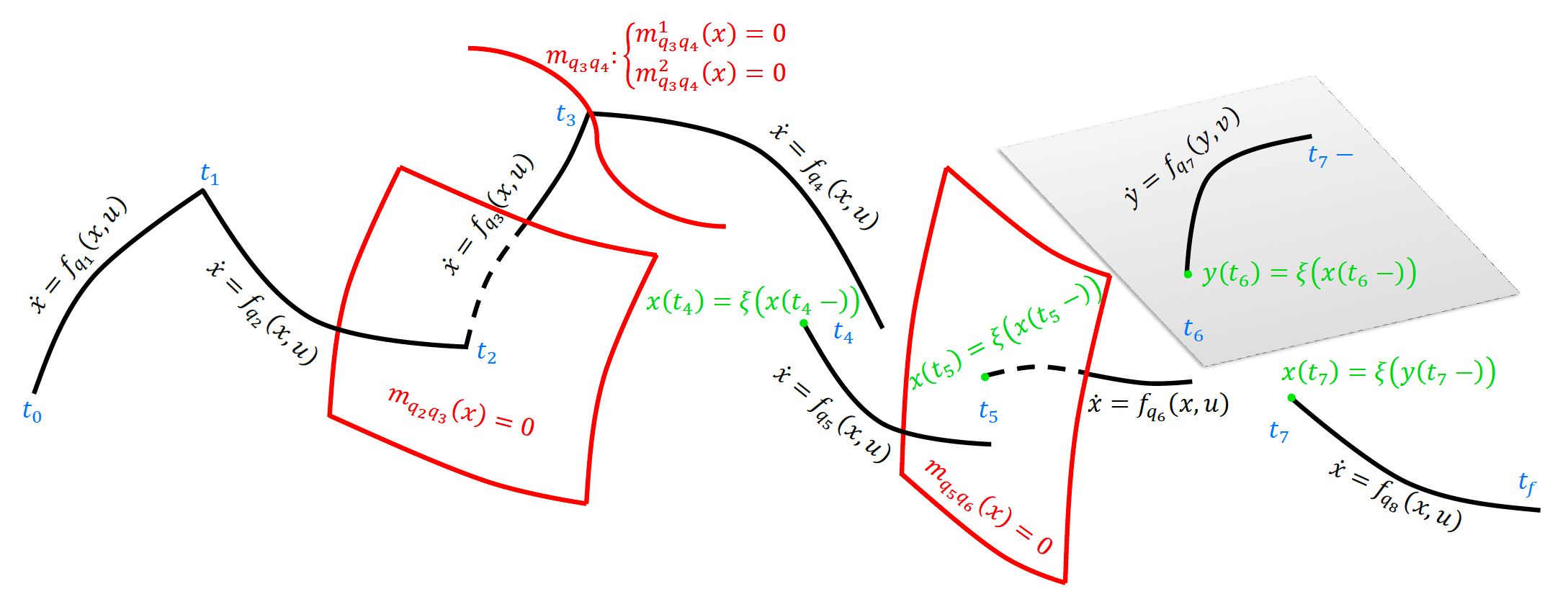
A hybrid system is a dynamic system that exhibits both continuous and discrete dynamic behavior. An iconic picture of a trajectory for a hybrid systems with both autonomous and controlled switchings and jumps is illustrated in this figure.
Show Description/Hide
During the continuous evolution of the system, the dynamics of the continuous (valued) state $x$ is governed by vector fields which are labled by discrete state $q$ and controlled by the continuous (valued) control input $u$
$$
\dot{x}_{q_{i}}\left(t\right)=f_{q_{i}}\left(x_{q_{i}}\left(t\right),u\left(t\right)\right),\;\;\;a.e.\;\;\, t\in\left[t_{i},t_{i+1}\right).
$$
At a switching instant $t_i$, the discrete input $\sigma$ controls the updates the discrete state
$$
q\left({t_{i}}\right)=\Gamma\left(q\left({t_{i}-}\right),x_{q_{i-1}} (t_{i}-),\sigma_{q_{i-1} q_{i}}\right) \, ,
$$
and the jump transition map $\xi$ determines the boundary conditions for the contnuous state
$$
x_{q_{i}}\left(t_{i}\right)=\xi_{\sigma_{q_{i-1} q_{i}}}\left(x_{q_{i-1}}\left(t_{i}-\right)\right)\equiv\xi_{\sigma_{q_{i-1} q_{i}}}\left(\underset{t\uparrow t_{i}}{\lim\,}x_{q_{i-1}}\left(t\right)\right) \, .
$$
The evolution of the system is considered to be known at an initial time
$$
h_{0}=\left(q_{0},x_{q_{0}}\left(t_{0}\right)\right)=\left(q_{0},x_{0}\right) \, .
$$
In our considered framework, switching manifolds corresponding to autonomous switchings and jumps are allowed to be codimension $k$ submanifolds in $\mathbb{R}^n$ with $1 \leq k \leq n$ (see also
[C12]), i.e. switching manifolds are described locally by
$$m_{q_{i-1} q_i}=\left\{ x: m_{q_{i-1} q_i}^{1}\left(x\right)=0 \land \cdots \land m_{q_{i-1} q_i}^{k}\left(x\right)=0 \right\} \,. $$
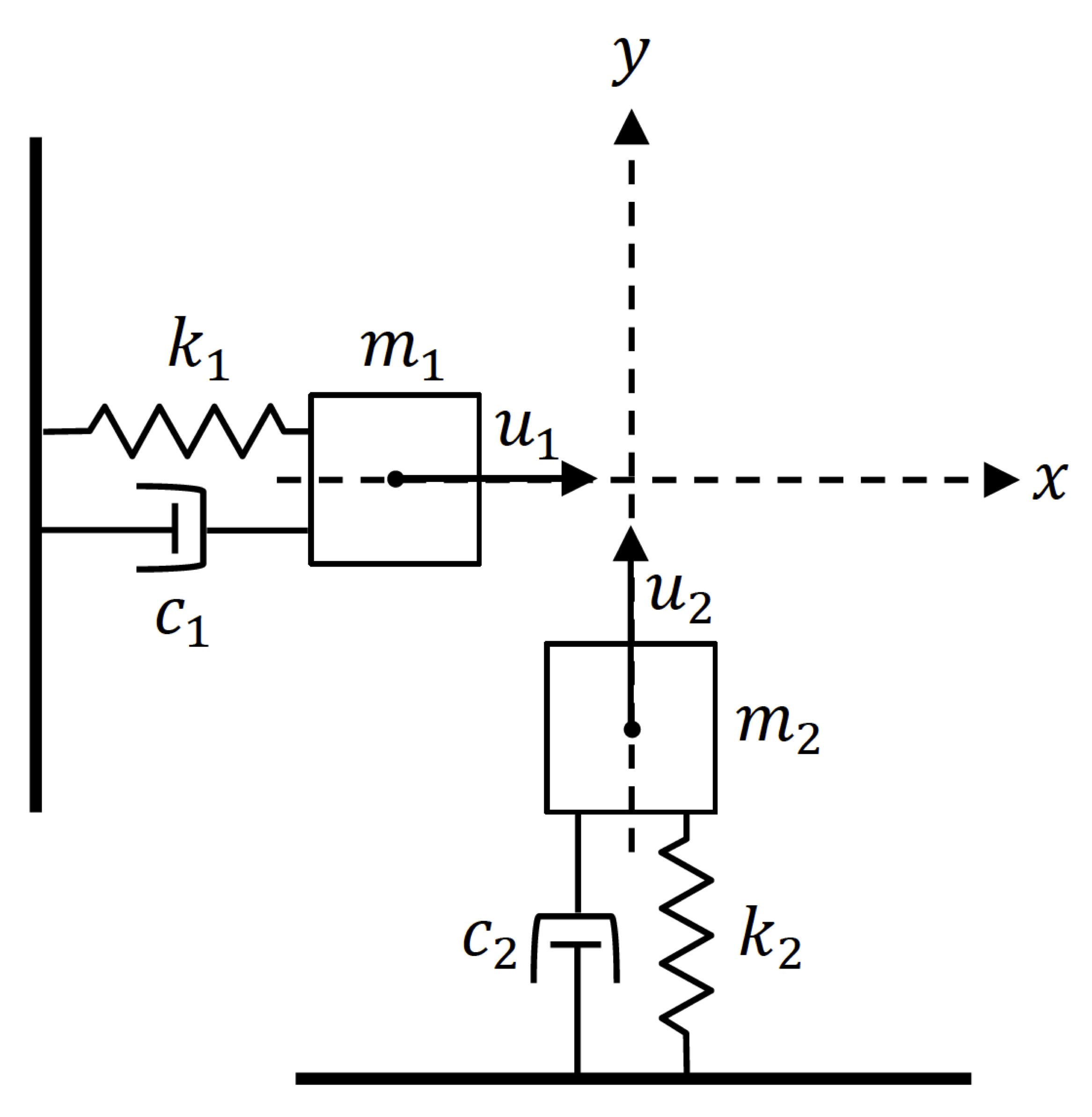
In the above figure, $t_3$ cooresponds to such a switching event. An example of an autonomous switching with low dimensional switching manifold is shown below, where in order for the masses to collide and therefore change the system's dynamics, both their horizental and vertical positions must be the same at the same time.
In addition, our framework permits the study of hybrid system that experience changes in the dimension of their state space at switching instants (see also
[C11]). Such a situation is illustrated at the instants $t_6$ and $t_7$ in the top figure.
Hybrid Optimal Control Problem:
Show Description/Hide
The cost to be infimized in the hybrid optimal control problem consists of running costs $l_{q_{i}}$, switching costs $c_{\sigma_{q_{i-1}q_{i}}}$ and a terminal cost $g$.
$$J\left(t_{0},t_{f},h_{0},L;I_{L}\right)= \sum_{i=0}^{L}\int_{s=t_{i}}^{t_{i+1}}l_{q_{i}}\left(x_{q_{i}}\left(s\right),u\left(s\right)\right)ds +\sum_{i=1}^{L}c_{\sigma_{q_{i-1}q_{i}}}\left(x_{q_{i}}\left(t_{i}-\right)\right)
+g\left(x_{q_{L}}\left(t_{f}\right)\right) \, .
$$
The cost-to-go is then formed as
$$
J\left(t,q,x,L-j+1;I_{L-j+1}\right)=\int_{t}^{t_{j}}l_{q}\left(x,u\right)ds
+\sum_{i=j}^{L}c_{\sigma_{q_{i-1}q_{i}}}\left(t_{i},x_{q_{i-1}}\left(t_{i}-\right)\right) +\sum_{i=j}^{L}\int_{t_{i}}^{t_{i+1}}l_{q_{i}}\left(x_{q_{i}}\left(s\right),u\left(s\right)\right)ds+g\left(x_{q_{L}}\left(t_{f}\right)\right) \, ,
$$
and the value function is defined as
$$
V\left(t,q,x,L-j+1\right)= \inf_{I_{L-j+1}} J\left(t,q,x,L-j+1;I_{L-j+1}\right)
$$
Hybrid Minimum Principle (HMP):
Show Description/Hide
Define the family of system Hamiltonians as
$$ H_{q_{j}}\left(x,\lambda,u\right)=\lambda^{T}f_{q_{j}}\left(x,u\right)+l_{q_{j}}\left(x,u\right)
$$
Then along an optimal trajectory $h^o=\left(q^{o},x^{o}\right)$, there exists an
adjoint process $\lambda^{o}$ such that
\begin{align}
\dot{x}^{o} &=\frac{\partial H_{q^{o}}}{\partial \lambda}\left(x^{o},\lambda^{o},u^{o}\right), \label{x dynamics}
\\
\dot{\lambda}^{o} &=-\frac{\partial H_{q^{o}}}{\partial x}\left(x^{o},\lambda^{o},u^{o}\right),\label{lambda dynamics}
\end{align}
almost everywhere $\; t\in\left[t_{0},t_{f}\right]$, with
\begin{align}
x^o\left(t_0\right) &=x_0,\\
x^o\left(t_{j}\right) &=\xi\left(x^o\left(t_{j}-\right)\right),\\
\lambda^{o}\left(t_{f}\right) &=\nabla g\left(x^{o}\left(t_{f}\right)\right),\label{lambda final condition}\\
\lambda^{o}\left(t_{j}-\right)\equiv\lambda^{o}\left(t_{j}\right) &=\nabla\xi^{T}\lambda^{o}\left(t_{j}+\right)+p\nabla m+\nabla c,\label{lambda boubdary condition}
\end{align}
where $p\in\mathbb{R}$ when $t_{j}$ indicates the time of an autonomous
switching, and $p=0$ when $t_{j}$ indicates the time of a controlled
switching. Moreover,
\begin{equation}
H_{q^{o}}\left(x^{o},\lambda^{o},u^{o}\right)\leq H_{q^{o}}\left(x^{o},\lambda^{o},u\right)\label{HminWRTu}
\end{equation}
for all $u\in U$, that is to say the Hamiltonian is minimized with respect to the control input, and at a switching time $t_{j}$ the Hamiltonian
satisfies
\begin{equation}
H_{q^o_{j-1}} \left. \left(x^{o},\lambda^{o},u^{o}\right)\right|_{t_{j}-} \equiv H_{q^o_{j-1}} \left(t_{j}\right)=H_{q^o_{j}} \left(t_{j}\right) \equiv H_{q^o_{j}}\left. \left(x^{o},\lambda^{o},u^{o}\right)\right|_{t_{j}+}\label{Hamiltonian jump}
\end{equation}
In addition to the consideration of switching costs (see e.g.
[C4]) as well as jump maps at the switching instants (see e.g.
[J4, C7, C8, C10 - C13]) in our considered framework, we further generalized the results of the HMP to cover the classes of hybrid systems whose autonomous and controlled state jumps at the switching instants are accompanied by changes in the dimension of the state space
[C11] and whose switching manifolds are codimension $k$ submanifolds in $\mathbb{R}^n$ with $1 \leq k\leq n$
[C12].
Hybrid Dynamic Programming (HDP):
Show Description/Hide
With the formation of the family of system Hamiltonians as
$$
H_q\left(x, \frac{\partial V}{\partial x},u\right):= l_{q}\left(x,u\right)+\left\langle \frac{\partial V}{\partial x},f_{q}\left(x,u\right)\right\rangle
$$
it is shown that the Hamilton-Jacobi-Bellman (HJB) equation holds
$$
-\frac{\partial V}{\partial t} = \inf_{u}\left\{ l_{q}\left(x,u\right)+\left\langle \nabla_{x}V,f_{q}\left(x,u\right)\right\rangle \right\},\;\;\;\; a.e.\; t \in \left[t_0,t_f\right],
$$
subject to the terminal condition
$$
V\left(t_{f},q_{L},x,0\right)=g\left(x\right),
$$
and at the switching times $t_i \in \tau_L = \left\{t_1, \cdots, t_L\right\}$ subject to the boundary conditions
$$
V\left(t_{j},q,x,L-j +1\right) = \min_{ \sigma_{j}\in\Sigma_{j}} \left\{ V \left( t_{j},\Gamma \left(q , \sigma_{ j}\right) ,\xi_{ \sigma_{j}} \left(x\right) ,L - j\right) + c_{ \sigma_{j}} \left(t_{j},x\right) \right\},
$$
and
$$
\hspace{-100mm} l_{q}\left(x,u^o\left(t_{j}-,x\right) \right)+\left\langle \nabla_{x}V,f_{q}\left(x,u^o\left(t_{j}-,x\right)\right)\right\rangle
\equiv -\frac{\partial}{\partial t} V \left(t_j -, q,x,L-j+1\right)
\\
\hspace{50mm} = -\frac{\partial}{\partial t} V \left(t_j -, \Gamma \left(q, \sigma_j\right) ,\xi_{\sigma_{j}}\left(x\right),L-j\right)
\equiv l_{\Gamma\left(q, \sigma_j\right)}\left(x,u^o\left(t_{j},\xi_{\sigma_{j}}\left(x\right)\right) \right)
+\left\langle \nabla_{x}V,f_{\Gamma\left(q, \sigma_j\right)}\left(x,u^o\left(t_{j},\xi_{\sigma_{j}}\left(x\right)\right)\right)\right\rangle,
$$
where if $t_{j}$ is a time of a controlled switching then $\Sigma_{j} = \Sigma$ subject to the automaton constraint that $\Gamma\left(q, \sigma_j\right)$ is defined; and in the case of an autonomous switching, the set $\Sigma_{j}$ is reduced to a subset of discrete inputs which are consistent with the switching manifold condition $m_{q,{\Gamma\left(q, \sigma_j\right)}}\left(x\right)=0$.
The Relation between the HMP and HDP:
In contrast to classical optimal control theory, the relation between the Minimum Principle and Dynamic Programming in the hybrid systems framework has been the subject of limited number of studies. We showed in
[J4, C13, C8] that along an optimal trajectory, $\nabla V$ which is the gradient of the value function in HDP, satisfies the same set of differential equations and have the same terminal and boundary conditions as the adjoint process for its corresponding trajectory, i.e.
$$
\frac{d}{dt}\nabla V=-\frac{\partial}{\partial x}f_{q^{o}}\left(x^{o},u^{o}\right)^T \nabla V-\frac{\partial}{\partial x}l_{q^{o}}\left(x^{o},u^{o}\right),
$$
$$
\nabla V\left(t_{f},q^{o},x\left(t_{f}\right),0\right)=\nabla g\left(x^{o}\left(t_{f}\right)\right),
$$
$$
\nabla V\left(t_{j}-,q_{j-1},x\left(t_{j}-\right),L-j+1\right)
=\left.\nabla\xi\right|_{x\left(t_{j}-\right)}^{T}\nabla V\left(t_{j}+,q_{j},x\left(t_{j}+\right),L-j\right)
+p\left.\nabla m\right|_{x\left(t_{j}-\right)}+\left.\nabla c\right|_{x\left(t_{j}-\right)} \, .
$$
Hence, the adjoint process and the gradient of the value function are equal almost everywhere, i.e.
$$
\lambda^{o}=\nabla V.
$$
The above argument was initially proved in
[C8] by the derivation of the boundary conditions for $\nabla V$ via variations over optimal trajectories, and the derivation of the dynamics and terminal conditions following the classical proof methods for the MP - DP relationship. In a consequent paper submitted to HSCC 2016
[C13] we provided a new proof method for the derivation of the dynamics that relaxes the strong requirement of the reachability of optimal trajectories in an open neighbourhood of a reference trajectory, that appears in classical proof methods. Our proof in
[C13] is based on the open denseness of the set of differentiability points of the value function which is allowed to be violated on a set of measure zero.
In the paper submitted to the IEEE Transactions on Automatic Control
[J4], a different approach is made in which the variations are studied over general trajectories which are not necessarily optimal. This provides the study of the evolution of the cost sensitivity along a general trajectory corresponding to a general control input with an admissible set of discontinuities. Namely, the cost sensitivity is govenred by
$$
\frac{d}{dt}\nabla J=-\left( \left[ \frac{\partial f_{q}\left(x,u\right)}{\partial x} \right]^T \nabla J +\frac{\partial l_{q}\left(x,u\right)}{\partial x}\right) \, ,
$$
and is subject to the terminal condition
$$
\nabla J\left(t_{f},q_L,x,0\right)=\nabla g\left(x\right) \,,
$$
and the boundary conditions
$$
\nabla J\left(t_{j},q_{j-1},x,L-j+1;I_{L-j+1}\right)
=\nabla\xi_{\sigma_j}^{T}\nabla J\left(t_{j}+,q_{j}, \xi_{\sigma_j} \left(x\right),L-j;I_{L-j}\right)
+p\nabla m+\nabla c
$$
with $p=0$ when $t_{j}$ indicates the time of a controlled switching and
$$
p=\frac{\left[\nabla J\left(t_{j},q_{j},\xi_{\sigma_{j}}\left(x\right),L-j;I_{L-j}\right)\right]^{T}\left(f_{q_{j}}\left(\xi_{\sigma_{j}}\left(x\right),u\left(t_{j}\right)\right)-\nabla\xi f_{q_{j-1}}\left(x,u\left(t_{j}-\right)\right)\right)+l_{q_{j}}\left(\xi_{\sigma_{j}}\left(x\right),u\left(t_{j}\right)\right)-l_{q_{j-1}}\left(x,u\left(t_{j}-\right)\right)}{\nabla m^{T}f_{q_{j-1}}\left(x,u\left(t_{j}-\right)\right)}
$$
when $t_{j}$ indicates the time of an autonomous switching.
To be completed soon...
To be completed soon...