 |
 |
| (a) Input. | (b) |
In this technical report, we present ongoing work to the problem of range synthesis for 3D environment modeling. We propose an efficient algorithm for extrapolating sparse range data to provide a dense 3D environment model. The extraction of range data from intensity images has been one of the key problems for computer vision, as addressed by numerous ``shape-from'' methods. Many of these methods provide incomplete data. More prosaically, while laser range sensors (for example based on LIDAR) have become well-established technology they are costly and often return data that is sparse relative to video images (most typically providing only dimensional-stripes of range data). In robotics, for example, the use of range data for navigation and mapping has become a key methodology, but it is often hampered by the fact that range sensors that provide complete (2-1/2D) depth maps with a resolution akin to that of a camera, are prohibitively costly.
Our method for range synthesis consists in using a statistical learning method for interpolating/extrapolating range data from only one intensity image and a relatively small amont of range data and without strong a priori assumptions on either surface smoothness or surface reflectance.
We base our range estimation process on inferring a statistical relationship between intensity variations and existing range data. This is elaborated using Markov Random Field (MRF) methods akin to those used in texture synthesis.
A single range value at a time is estimated where only intensity is known. This is done by using neighboring locations where both range and intensity data is available.
We use Markov Random Fields (MRF) as a model that captures characteristics of the relationship between intensity and range data in a neighborhood of a given voxel, i.e. the data in a voxel are determined by its immediate neighbors (and prior knowledge) and not on more distant voxels (the locality property). The other property that we exploit is limited stationarity, i.e. different regions of an image are always perceived to be similar. This property is true for textures but not for more general classes of images representing scenes containing one or more objects. In our algorithm, we synthesize a depth value so that it is locally similar to some region not very far from its location. The process is completely deterministic, meaning that no explicit probability distribution needs to be constructed.
(Note: the algoritmh is explained in the report file: report_abril.ps.gz)
In our algorithm we synthesize one depth value at a time. The order in which we choose the next depth value to synthesize will reflect the final result. We have implemented different scan orderings for assigning depth values. These are:
In this initial work we estimate the depth values where missing by using the already existing range values. Although this does not always represent the true range, we have found that our experimental results are quite satisfactory.
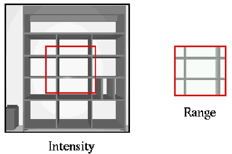
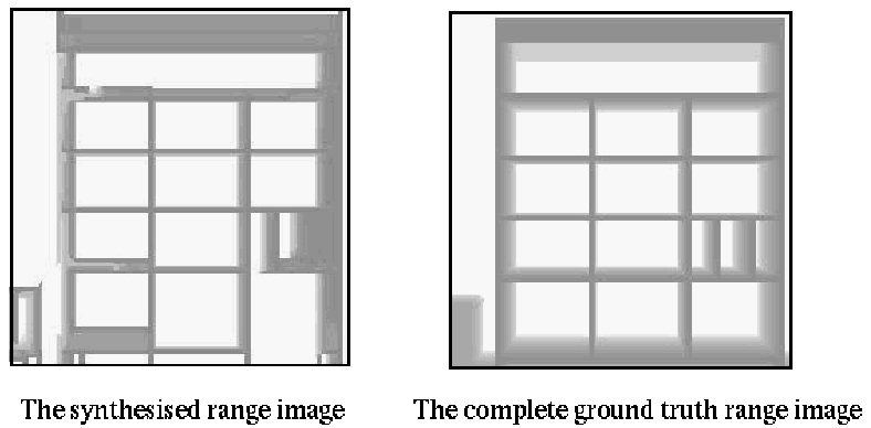
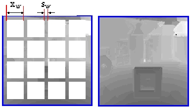
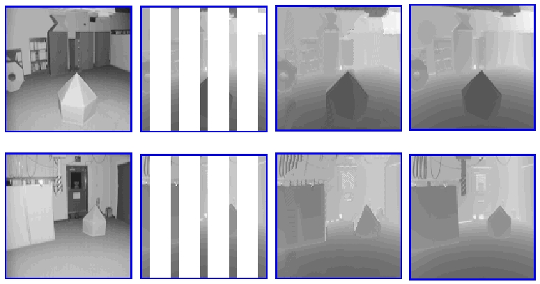
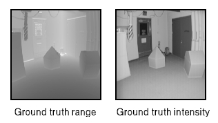
We have tested our algorithm using synthetic and real data. The synthetic data were generated with the 3D rendering package PovRay using natural lighting conditions. In the left side of Figure 1a, a synthetic intensity image of an empty bookshelf is shown; the subwindow in the right side is the associated range image taken from the position indicated by the red rectangle in the intensity image. These images are given as an input to our algorithm. For this case, the size of the neighborhood is set to be 9x9 pixels. The left side of Figure 1b shows the range synthesis results, and to the right, as a way of visual comparison, the complete synthetic range data is shown. It can be seen that the algorithm captures most of the changes involved in the intensity information and are reflected in the range synthesis process.
|
|
| (a) Input. | (b) |
Figure 1. Results of range synthesis on synthetic data. Panel (b) shows the comparison of synthesized range with ground truth for this artificial scene.
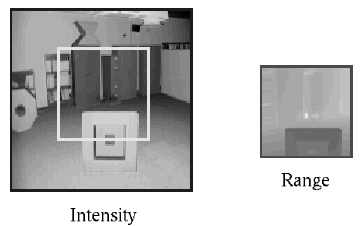
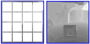
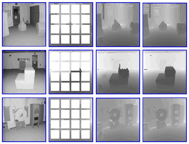
Representative results based on data acquired in a real-world environment are shown in Figures 2 through 9. The real intensity (reflectance) and range images of indoor scenes were acquired by an Odetics laser range finder mounted on a mobile platform. Images are 128x128 pixels and encompass a 60x60 degrees field of view. As with the synthetic data, we start with the complete range data set as ground truth and then hold back most of the data to simulate the sparse sample of a real scanner and to provide input to our algorithm. This allow us to compare the quality of our reconstruction with what is actually in the scene. In the following we will consider two strategies for subsampling the range data.
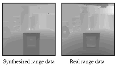
The first type of experiment involves the range synthesis when the initial range is a window of size pxq and at position (r_x,r_y) on the intensity image. Figure 2a shows the intensity image (left) of size 128x128 and the initial range (right), a window of size 64x64, i.e. only the 25% of the total range is known. The size of the neighborhood is 5x5 pixels. The synthesized range data obtained after running our algorithm is shown in the left side of Figure 2b; for purposes of comparison, we show the complete real range data (right side).
It can be seen that the synthesized range is very similar to the real range. The Odetics LRF uses perspective projection, so the image coordinate system is spherical. To calculate the residual errors, we first convert the range images to the Cartesian coordinate system (range units) by using the equations in~\cite{Storjohann90}. For this example, the average residual error is 7.98.
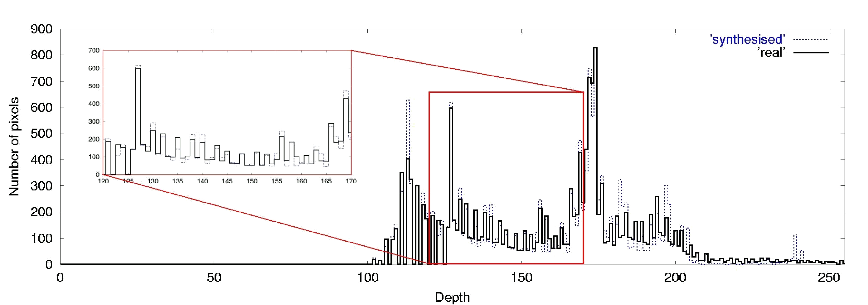
In the second type of experiment, the initial range data is a set of stripes with variable width along the x- and y-axis of the intensity image. We tested with the same intensity image used in the previous section in order to compare both results. Two experiments are shown in Figure 3. The initial range images are shown in the left column, and to their right are synthesized results. In Figure 3a, the width of the stripes s_w, is 5 pixels, and the area with missing range data (x_w x x_w) is 25x25 i.e., 39% of the range image is known. For Figure 3b, the values are s_w=3, x_w=28, in this case, only 23% of the total range is known. The average residual error (in range units) for the reconstruction are 2.37 and 3.07, respectively. In Figure 4 a graph of the density of pixels at different depth values (scale from 0 to 255) of the original and synthesized range of Figure 3a. Figure 5 displays two different views using the real range and the synthesized range results of Figure 3.
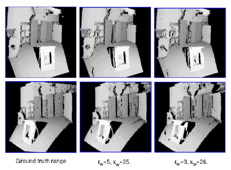
The results are surprisingly good in both cases. Our algorithm was capable of recovering the whole range of the image. We note, however, that results of experiments using stripes are much better than those using a window as the initial range data. Intuitively, this is because the sample spans a broader distribution of range-intensity combinations than in the local window case.
Our algorithm was tested on $30$ images of common scenes found in a general indoor man-made environment. Two cases of subsampling were used in our experiments. Case 1 is as one of the subsampling previously described, with r_w=5 and x_w=25, applied along x- and y-axis. In Figure 6a, we show 3 more examples of this case, the average residual errors are, from top to bottom, 2.84, 4.53 and 3.32. For Case 2, r_w=8 and x_w=22, but applied only along the x-axis. Figure 6b shows two examples of this case. Here the average residual errors are 4.17 and 5.25, respectively. Once again, it can be seen that the results are good in both cases. The maximum average residual errors obtained from all 30 test images were for Case I, 6.52 and for Case II, 11.85.
To see the results for both cases of the 30 examples go to the following links: case1 and case2.
It is important to note, that the initial range data given as an input is crucial to the quality of the synthesis, that is, if no interesting changes exist in the range and intensity, then the task becomes difficult. However, the results presented here demonstrate that this is a viable option to facilitate environment modeling.
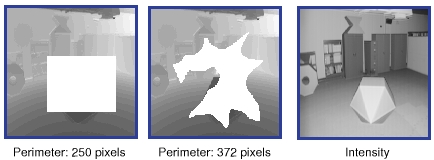
We now show some experiments where the missing range is of arbitrary shape. The input parameters are the left superior coordinates and the size in x- and y-axis of the maximum rectangle that surrounds the arbitrary shape.
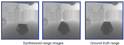
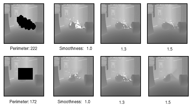
Our hypothesis is that the less compact the shape that contains the missing range the better the range estimation. We show this in the following figures. In Figure 7a, two input range images (the left and middle images) and input intensity are given. Both range images have the same area, which is 3864 pixels, but different shapes and perimeters, 250 and 372 pixels, respectively. Figure 7b shows the synthesized range images (left and middle) and the ground truth range image for comparison purposes. The residual average errors are 7.17 and 3.99, respectively.
We now show how the amount of input range affects the estimation of range where missing. In Figure 8a we show some of the input range images, the white squares represent the area of missing range, which varies from 12100 (110x110) to 100 pixels. The synthesized results are shown in Figure 8b.
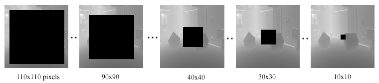
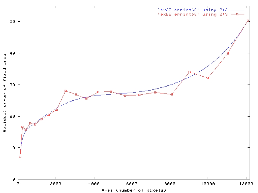
We calculate the residual average error of each synthesized image but only in a fixed area in order to be able to evaluate the range synthesis process. This fixed area is the 10x10 square show in the rightmost image of Figure 8a. In Figure 9, we plot the residual average error of each synthesized image versus the amount of missing range.
Size of the mask (neighborhood): The size of the neighborhood plays an important role in the range synthesis process. If it is too small then we may find many similar neighborhoods since it does not capture much about the relationship between the intensity and range. If it is too large then it may be difficult to find a similar neighborhood at all, since we are dealing with multiple objects of different sizes in the scene. It is also important to consider the amount of range that is available initially. In cases where we have a very sparse range available, the size of the mask will be set by the width of the stripes of available range, as were the case in the experiments shown.
Size of the area where looking for the best match: This is another aspect that needs to be considered. Neigborhoods that are located at a close distance from the voxel to be synthesized are more probable to contain similarity information in both intensity and range than neighborhoods located far away. This parameter will help to reduce the running time of our algorithm.
Order of the estimation (spiral, maximum number of neighbors):As it was already mentioned, the order in which the depth values are assigned influences in the quality of the estimation process.
The estimation of range values: Currently, the estimation range values is done by selecting the range value of that voxel with the most similar neighborhood to the voxel to be synthesized. However this range value may not suitable for cases in which the normal direction in the z-axis of the surface containing the voxel to be synthesized is one. In the next Part, we are dealing with this problem.
As it was described in Part I, we were not assigning new depth values to the voxels with missing range, i.e. only the already existing values were considered in the algorithm. However, if we want to have a realistic range synthesis, we need to consider additional information to be able to compute new depth values based on the available information. In Part II, we now consider the surface normals as additional information. Surface normals give the orientation of a given surface and if there exists a voxel which belongs also to this surface, but its depth value is missing, then we can use its surface normal to estimate its new depth value.
We use the eigenvalue method to compute surface normals. In this method, we find the eigenvectors and their correspondent eigenvalues of a surface patch. The two eigenvectors corresponding to the two largest eigenvalues are the two tangent vectors which determine the tangent plane to the surface patch, while the eigenvector corresponding to the smallest eigenvalue is pointing in the normal direction.
For comparison reasons, we are using the same set of range and intensity data and carrying on the same type of experiments as in Part I, with the only difference that now we are estimating first the surface normals and then the new depth values.
We now show some experiments where the missing range is of arbitrary shape. The input parameters are the left superior coordinates and the size in x- and y-axis of the maximum rectangle that surrounds the arbitrary shape.
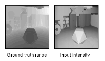
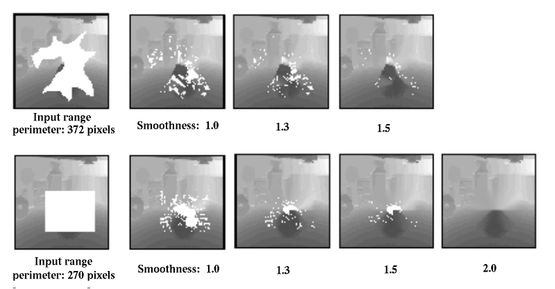
Figure 10a shows the ground truth range and input intensity images. In Figure 10b, two input range images are shown in the left column. Both missing (white) areas have the same area, which is 3864 pixels, but different shapes and perimeters, 250 and 372 pixels, respectively. The synthesized images are shown in the rest of the columns, each of them with its respective smoothness value used in the calculation of the new depth values. (explain later) Another example is shown in Figure 11. In this case the missing (white) areas have an area of 1824 pixels, and perimeters of 222 and 122 pixels, respectively.
White pixels on the following figures mean that surface normals at that location were not possible to compute therefore the new depth value was not calculated.
White pixels on the following figures mean that surface normals at that location were not possible to compute therefore the new depth value was not calculated.
Size of the cluster (mask) used for calculating the normals.
The co-normality threshold (alpha): When calculating the surface normal and when doing the normal estimation.
Calculation of the new depth values